Error Correction with Hamming Codes

Introduction to Bit-level Error Checking

In my last post, we discussed how parity is used for bit-level error checking. Here’s a quick review of how that works:

Parity is the state of being even or odd. A parity bit is used to note how many 1’s are expected in a sequence of bits. Generally an even parity bit is used, meaning the parity bit will assume a value of 1 if the bit sequence has an odd number of 1’s, making the total parity even, or a value of 0 if the bit sequence already has an even number of 1’s, maintaining the already even parity. Once data gets transferred, it can be checked for errors by comparing the parity bit to the number of 1’s in the data. If the total number of 1’s, including the parity bit, is no longer even, then something went wrong.

The downfall of using parity bits as described above is that you will not know if an even number of errors has occurred, which would go undetected using parity in this way. Additionally, should an error be detected, you will not know where in the data it occurred.

In this blog post, we will take a look in Hamming Codes and how they make use of parity bits in such a way that allows both detection and correction of single-bit errors, and detection of up to two errors.

What are Hamming codes?

Hamming codes were invented by Richard Hamming as a result of frustration from knowing that errors had occurred in his data but not knowing where the errors were.

Before we get into his solution to that problem, let’s consider what possibilities exist for performing error correction. We saw above what a single parity bit can do, which, while helpful to an extent, is relatively limited. There’s the option for redundancy, which could be used in itself to compare multiple instances of data to find unexpected bit flips based on the greater number of 1’s or 0’s. Redundancy, however, always comes at a cost of storage. For every redundant usage of storage, there is less storage for new data.

So to that we may ask, how can we minimize the amount of space required for error checking while providing even more knowledge about what happened to corrupted data?

And that is exactly where Hamming codes come in.

Hamming codes utilize a mathematically relevant number of parity bits for both error checking and error correction. In this blog post, we’re going to take a look into the (15,11) Hamming code specifically. This is just a name based on the data size we’ll be talking about and working with here; Hamming codes can work for larger data sizes as well.

How do Hamming codes work?

Hamming codes use a pre-determined (we’ll see how) number of parity bits such that those few bits can be used to determine when a single error occurs and exactly which bit had the unexpected flip. This method also works for knowing when not just one but two errors occurr.

We discussed earlier how a single parity bit for a sequence of data will alert a change in the data only if there exists an odd number of bit flips. Additionally, you cannot find out what bit(s) were changed. However, when you use multiple parity bits, you can gleam a lot more information.

Hamming codes use multiple parity bits to essentially split the data in multiple ways by allowing the ability to piece together which parity bits remain correct for their subset of data, and which parity bits do not match their expected data. The number of required parity bits is determined by the size of the data. For a given power of 2 number of bits, that power is the number of parity bits that will be used. We’ll walk through this with a 16-bit example, and it will become clear how it would work for any other quantity of data.

This is easiest to show and explain with actual data, so we’ll follow along an example. As mentioned, we’re going to look at a (15,11) Hamming code specifically. This is in reference to 15 total bits being used to include both 11 bits of actual data and 4 parity bits. 16 = 2^4, so there are 4 parity bits, following along what was said above.

Example

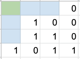
Let’s take the 11-bit sequence 01001101011.

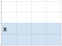
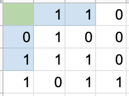
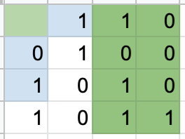
Because we’re working with 16 bits total, we’re going to use a 4x4 matrix. The parity bit locations are highlighted in blue, the locations of the 11 bits of data are not highlighted, and we’ll come back around to the green box.

First, we need to populate the data into this matrix. We do so chronologically starting in the top row, left to right, and down a row each time we hit the end of the previous row. It will look as follows:

Now, we can look to determine the parity bit values. The following pictures show what combination of rows or columns are included in each parity bit’s determining data, with x indicating which parity bit is used for that data:

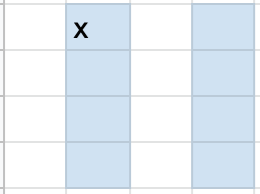
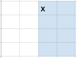
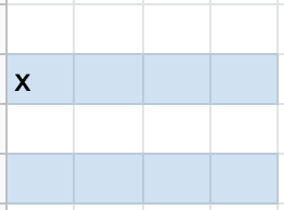
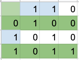
Now that we know what data is included for each parity bit, let’s determine the values of those parity bits. We’ll refer to the top row’s parity bits as parity bits 1 and 2, respectively, and the first column’s parity bits as parity bits 3 and 4, respectively.

We see for the parity bit in position 1 that there are 3 1’s in the included (2nd and 4th) columns, so this parity bit value will be 1. The same is the case for the second parity bit, with columns 3 and 4. Rows 2 and 4 have 4 1’s, making the third parity bit 0. Lastly, the fourth parity bit is a 1 to make the number of 1’s in rows 3 and 4 an even number. The resulting matrix looks as follows:

Now we can test it! Let’s change one bit in the data. Here’s what the altered matrix now looks like:

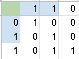
Let’s check each parity bit to see which ones don’t align with the data.

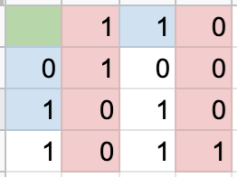
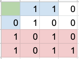
As we can see, parity bits 1 and 4 did not turn out the expected results. Because parity bit 2’s data was fine, we know something went wrong in column 2. And because parity bit 3’s data was fine, we know something went wrong in row 3. And there we have it, the flipped bit!

And now, as promised, we can talk about that pesky green square. What is it supposed to represent? Well, you may or may not have wondered what happens if there aren’t any errors. This is where the first bit comes in. It can be used to ensure even parity of the entire data sequence, which in turn is what allows the ability to detect two errors. If there were to be a single error, we saw above how the other four parity bits would figure that out. And of course, this extra parity bit would recognize that single error as well. Where it comes in handy is when a second error has occurred, leaving this parity unable to detect the two errors on its own. However, the other four parity bits would recognize that something was off, indicating that (at least) two errors occurred. To make this clearer, consider how parity works as described at the beginning of the post. A single parity bit will not pick up on even numbers of errors, as the parity will technically still be even. However, even if this is the case in our 4x4 matrix, the other four parity bits will still end up with errors due to the multiple instances of checking parity of their subsets.

Conclusion and Reference

I hope you found this post to be a cool follow-up from the last one!

The inspiration for this post was a video sent to me after publishing the last post about parity. It explains in greater detail everything that we went over in this post and is a great video for visually depicting how Hamming codes work. Check it out here: Hamming codes, how to overcome noise.